Robustness regions

library(bayesplay)

In typical Bayes factor analyses, a prior is specified for the alternative and null models. For example, an analyst might specify a normal distribution with a mean of 0 and standard deviation of 15 as the prior for the alternative model. In bayesplay syntax, this would be done as follows:

prior(family = "normal", mean = 0, sd = 15)

In specifying a prior in this way, the analyst chooses a set value for the two parameters (mean and standard deviation). It might be of interest to

The bayesplay package includes functionality for systematically varying parameters of the alternative prior for computing robustness regions and for visualizing these robustness regions.

data_model <- likelihood(family = "student_t", mean = 5, sd = 11, df = 12)
alternative_prior <- prior(family = "normal", mean = 0, sd = 15)
null_prior <- prior(family = "point", point = 0)

m1 <- data_model * alternative_prior
m0 <- data_model * null_prior

bf <- integral(m1) / integral(m0)

summary(bf)
#> Bayes factor
#>  Using the levels from Wagenmakers et al (2017)
#>  A BF of 0.6369 indicates:
#>  Anecdotal evidence

One might then wonder how robust this conclusion is to variations in the alternative prior. Would the conclusions change if a higher value or a lower value was selected for the standard deviation of the prior? With the bfrr function, it’s possible to set an upper and lower bound of the standard deviation and to compute and visualize the resulting Bayes factor for values within this range.

In the example below, the standard deviation is varied across the range from 1 to 20 (in steps of 1).

rr <- bfrr(
  likelihood = data_model, # reuse the definition above
  alternative_prior = alternative_prior, # reuse the definition above
  null_prior = null_prior, # reuse the definition above
  parameters = list(sd = c(1, 50)) # vary sd from 1 to 20
)

plot(rr)

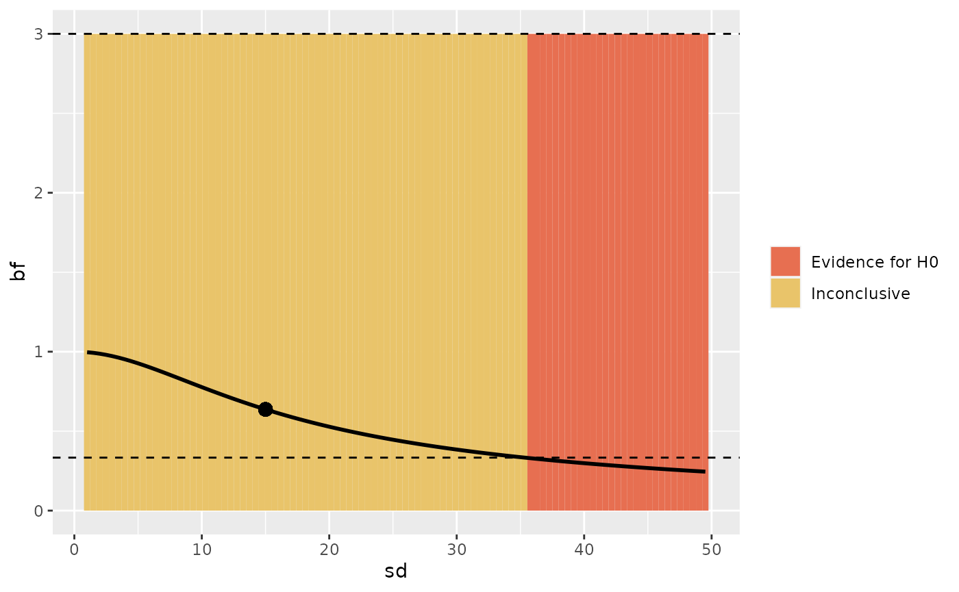
data_model <- likelihood(family = "noncentral_d", d = 0.2, n = 50)
alternative_prior <- prior(family = "cauchy", location = 0, scale = 1)
null_prior <- prior(family = "point", point = 0)

m1 <- data_model * alternative_prior
m0 <- data_model * null_prior

bf <- integral(m1) / integral(m0)

summary(bf)
#> Bayes factor
#>  Using the levels from Wagenmakers et al (2017)
#>  A BF of 0.2901 indicates:
#>  Moderate evidence

rr <- bfrr(
  likelihood = data_model, # reuse the definition above
  alternative_prior = alternative_prior, # reuse the definition above
  null_prior = null_prior, # reuse the definition above
  parameters = list(scale = c(0.1, 2))
)
rr
#> Prior robustness analysis:
#> 
#>   Alternative prior
#>   -----------------
#>     Family
#>       cauchy
#>     Parameters
#>       location: 0
#>       scale: 1
#> 
#>   Null prior
#>   -----------------
#>     Family
#>       point
#>     Parameters
#>       point: 0
#> 
#>   Likelihood
#>   -----------------
#>     Family
#>       noncentral_d
#>     Parameters
#>       d: 0.2
#>       n: 50
#> 
#>  The original parameters gave a Bayes factor of 0.29.
#> Using the cutoff value of 3, this result provides evidence for H0.
#> 
#> 1 parameter of the alternative prior was varied for the robutness analysis:
#>   The scale was varied from 0.1 to 2 (step size: 0.019)
#> 
#> Outcome
#> -----------------
#> 60 of 100 (0.6) tested priors provided evidence for H0 (BF < 0.33)
#> 
#> 0 of 100 (0) tested priors provided evidence for H1 (BF > 3)
#> 
#> 40 of 100 (0.4) tested priors were inconclusive (0.33 < BF < 3)
#> 
#> The conclusion of 'Evidence for H0' was robust over 0.6 tested priors
#> 
#> No tested priors gave the opposite conclusion
#> 

plot(rr)

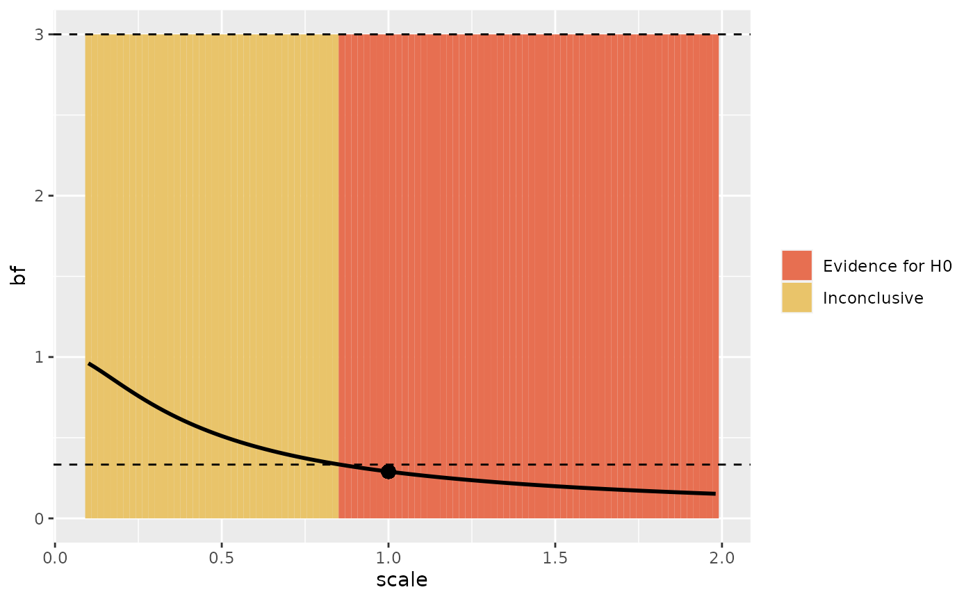
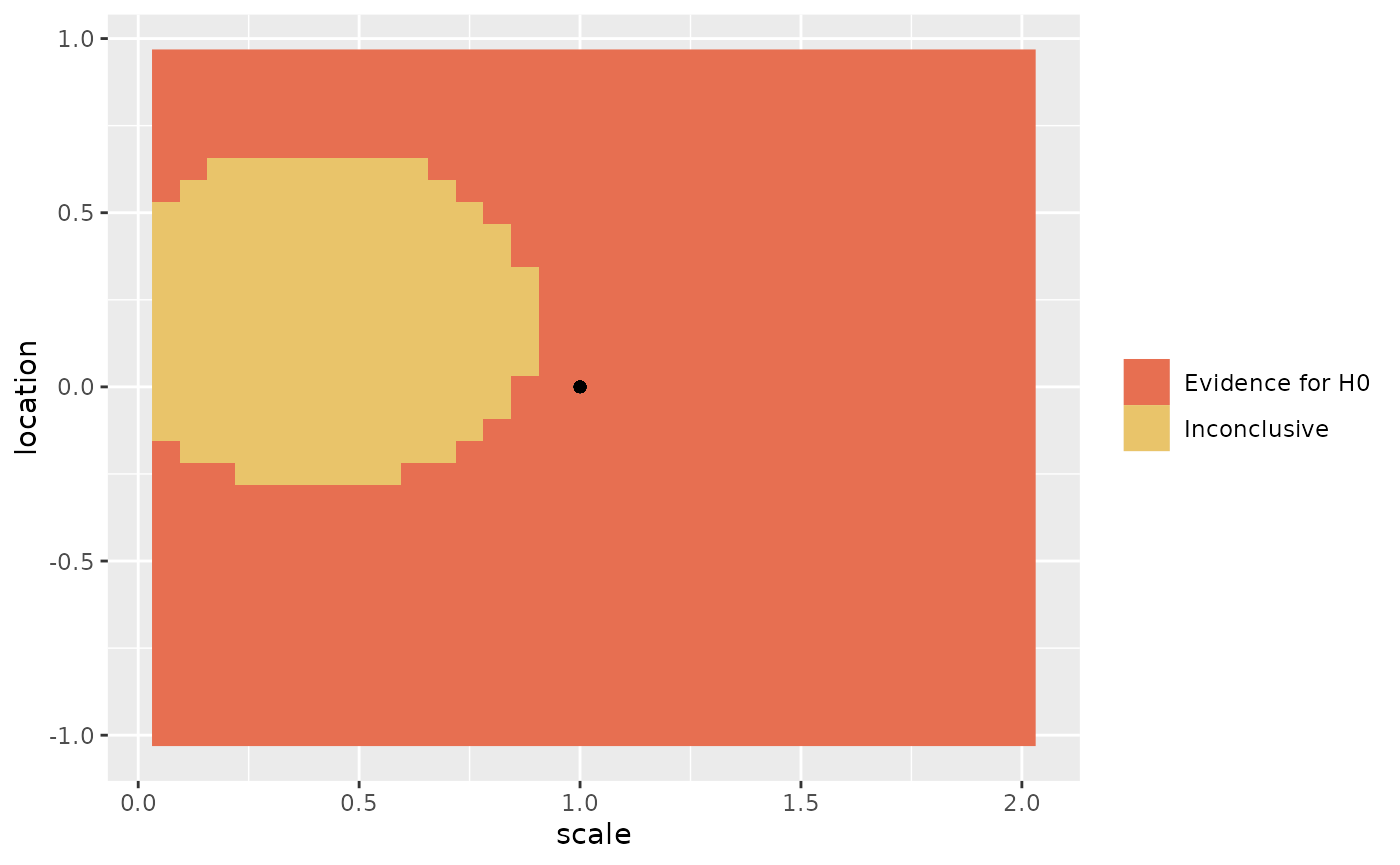
rr <- bfrr(
  likelihood = data_model, # reuse the definition above
  alternative_prior = alternative_prior, # reuse the definition above
  null_prior = null_prior, # reuse the definition above
  parameters = list(scale = c(0, 2), location = c(-1, 1)),
  steps = 32
)
rr
#> Prior robustness analysis:
#> 
#>   Alternative prior
#>   -----------------
#>     Family
#>       cauchy
#>     Parameters
#>       location: 0
#>       scale: 1
#> 
#>   Null prior
#>   -----------------
#>     Family
#>       point
#>     Parameters
#>       point: 0
#> 
#>   Likelihood
#>   -----------------
#>     Family
#>       noncentral_d
#>     Parameters
#>       d: 0.2
#>       n: 50
#> 
#>  The original parameters gave a Bayes factor of 0.29.
#> Using the cutoff value of 3, this result provides evidence for H0.
#> 
#> 2 parameters of the alternative prior were varied for the robutness analysis:
#>   The scale was varied from 0 to 2 (step size: 0.0625)
#>   The location was varied from -1 to 1 (step size: 0.0625)
#> 
#> Outcome
#> -----------------
#> 844 of 1024 (0.82) tested priors provided evidence for H0 (BF < 0.33)
#> 
#> 0 of 1024 (0) tested priors provided evidence for H1 (BF > 3)
#> 
#> 180 of 1024 (0.18) tested priors were inconclusive (0.33 < BF < 3)
#> 
#> The conclusion of 'Evidence for H0' was robust over 0.82 tested priors
#> 
#> No tested priors gave the opposite conclusion
#> 

plot(rr)